#Loads data from a CSV file into RStudio
LincsOCR <- read.csv("LincolnshireOCR.csv")

#Filters out all non 'Event' data

lincsEvents <- filter(LincsOCR, TYPE == 'EVENT')I was really looking forward to giving a paper at the International Medieval Congress at Leeds this year on text mining medieval court records on session 836 which was organised by Dr Claire Kennan and Dr Emma J. Wells. I had intended to use the process as an excuse to learn text mining using R. I thought it might be provide some material for my thesis and I am quite evangelical about the possibilities of text mining historical documents. For obvious reasons the Congress was cancelled but I still wanted to go ahead with the work and I thought I could share it via a blog post instead. This post is intended as an outline of some potential uses of text mining rather than an exhaustive step-by-step tutorial. At this point I should stress that I relied a lot on the generosity of the R community who make a lot of training materials available online for free and particularly on Text Mining with R which is available for free or can be purchased online.1
A Lincolnshire Records Society Volume was a good beginning point for learning text mining.2 This volume is well suited to digitisation thanks to the diligence of editor and translator Bernard McLane. The records which McLane edited are drawn from an investigation which took place in 1340 on the insistence of Edward III in the aftermath of a failed military campaign against the French crown in the Low Countries. They began as investigations of royal ministers who were suspected of enriching themselves at the expense of the crown and the populace during Edward’s absence. They ultimately expanded to include all offences and so the records concern a variety of alleged crimes. McLane estimated that 767 offences were carried out by officials and 325 by ordinary citizens. I set myself the goal of attempting to use text mining techniques to automatically categorise some of these offences according to my research themes. This post will outline some of the first steps that are generally taken when mining a document like this. Don’t worry too much about following the code in detail, the goal here is to highlight some of the possibilities of data science approaches when applied to medieval sources.
Preparing your data for analysis
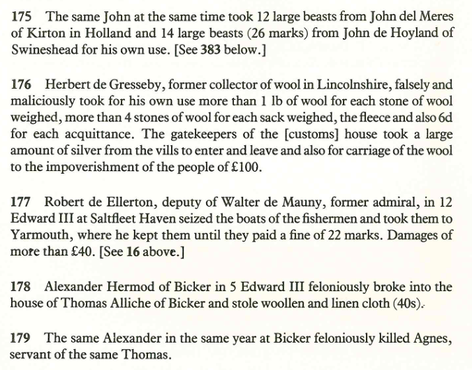
Above is an example of some of the allegations contained in the text. I scanned the entire volume, put it through some OCR software, and uploaded the data to the Recogito platform. This is provided by the Pelagios project and carries a useful interface which you can use to annotate text and images with XML, RDF, JSON, or KML. It can also perform ‘named entity recognition’ which extracts names and locations. If you want to you can also geocode the locations within Recogito. I found this aspect less useful because of the lack of an integrated gazetteer for medieval England (I harbour an ambition to build one). There is also a text editor in which you can manually tag personal names, locations, or events from your text. All of this data can be exported in a few different ways. Recogito is useful but not completely necessary. All of the steps can be carried out in other software or manually. I just found it has a lower barrier to entry and allowed me to focus on analysing the text.
I used the text editor to check the automated tagging, which required some correction, the most useful aspect of Recogito was tagging each individual entry as an event. This made it easier to carry out meaningful analysis and manipulation. After this I downloaded the data as a csv file and loaded it into R Studio for the text mining process. Firstly, I stripped out anything that wasn’t an ‘event’ or allegation with the filter() command. This is useful to extract sections of the data you are interested in working with.
Tokenisation
Luckily Bernard McLane labelled each entry on the court roll with a unique ID. I extracted the first word from each entry to create an index which would allow me to refer back to McLane’s volume. After this I took this data and broke it up into single word observations through a function called unnest_tokens(). This process is called tokenisation and each individual word, or set of digits, is refereed to as a token. This is useful for analysis of the corpus as a whole. This process removes all punctuation and puts the text into lower case. It is possible to unnest the data as bi grams (two word pairings) or even further but that is a job for another day. At this point the goal is just to uncover single words which I can then use to auto-label allegations as particular offences. After tokenization there were 4,739 unique words in the corpus.
#Tokenizes the text

lincsEventsTokens <- lincsEvents %>% unnest_tokens(word, QUOTE_TRANSCRIPTION)

#Unstopped plot


lincsEventsTokens %>% count(word, sort = TRUE) %>% filter(n > 200) %>% mutate(word = reorder(word, n)) %>% ggplot(aes(word, n)) + geom_col(fill="#ffd700") + xlab(NULL) + coord_flip() + theme_minimal()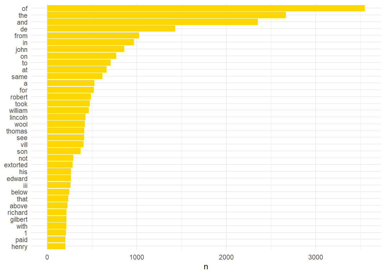
Stop Words
This plot only shows those words with a frequency of 200 or greater. An immediate problem is the prevalence of the most common words. Luckily this is an easy fix. Using the anti_join(stop_words) command we can remove these common words. This is a collection of frequently used English words and it was here I found myself particularly grateful that Dr McLane translated the records. There are of course equivalent versions for other languages although none, as far as I am aware, for medieval British Latin. Once these words are removed the plot looks quite different but no more useful.
#Removing 'stop words'
lincsStopped <- lincsEventsTokens %>% anti_join(stop_words)
Joining with `by = join_by(word)`#Data with stop words removed and plot >200
lincsStopped %>% count(word, sort = TRUE) %>% filter(n > 200) %>% mutate(word = reorder(word,n)) %>% ggplot(aes(word, n)) + geom_col(fill="#ffd700") + xlab(NULL) + coord_flip() + theme_minimal()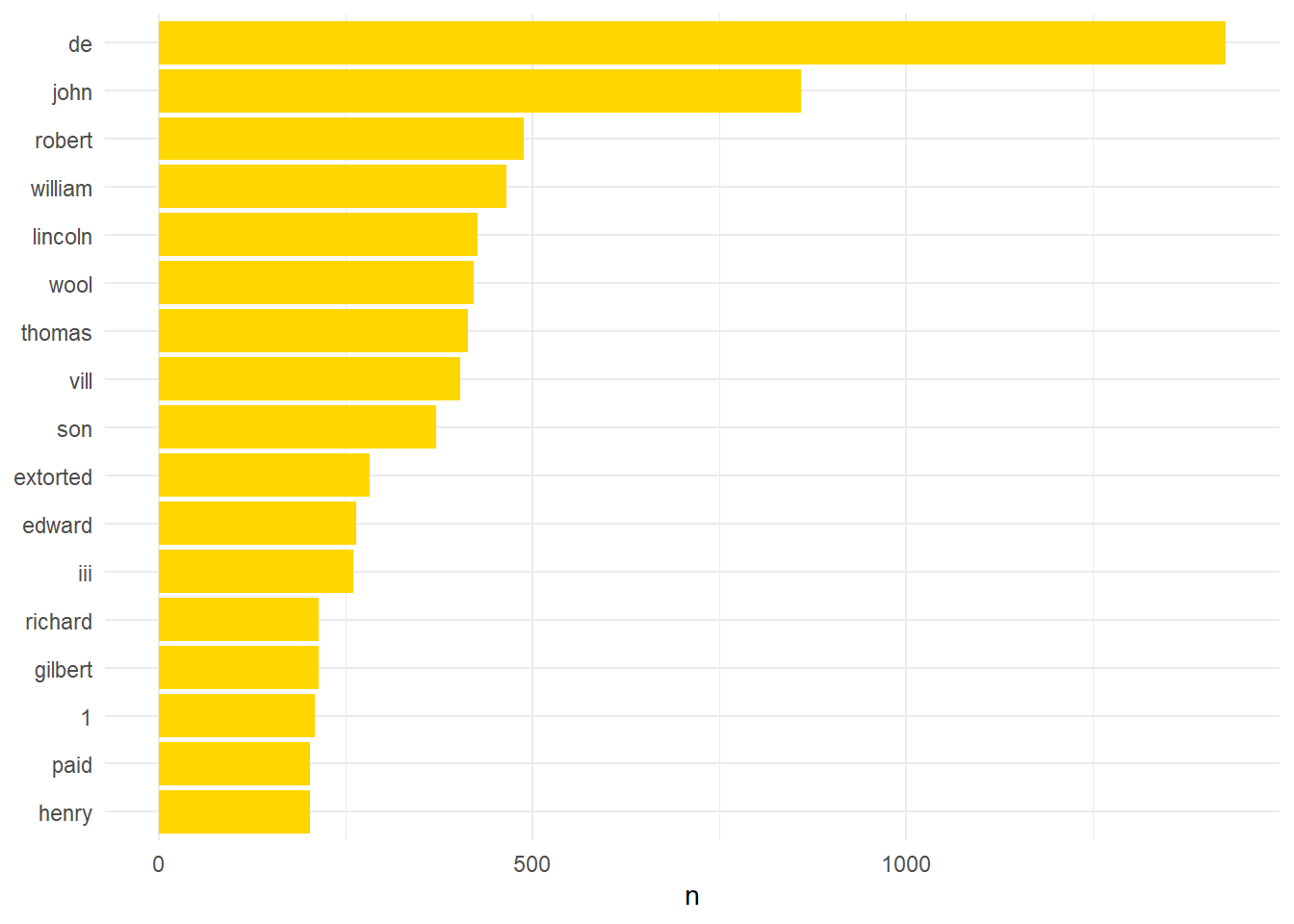
Applying the stop_words data takes the count of unique tokens down to 4,472. There is a prevalence of names, places, or other immaterial information. This is slightly harder to fix but as Recogito tags individuals I was able to use that information. The automated tagging was not perfect but I caught most of its mistakes in my read through.
#Create a list of Personal names from the original data
lincs_people <- filter(LincsOCR, TYPE == "PERSON")

#Select desired columns from original text
lincs_stop_people <- lincs_people %>% select(QUOTE_TRANSCRIPTION, TYPE, UUID)

#Unnest Tokens
lincs_stop_people <- lincs_stop_people %>% unnest_tokens(word, QUOTE_TRANSCRIPTION)

#Removing Personal name using anti_join()
lincs_people_stopped <- lincsStopped %>% anti_join(lincs_stop_people)
Joining with `by = join_by(UUID, TYPE, word)`#Plot with personal names removed and >150 occurences
lincs_people_stopped %>% count(word, sort = TRUE) %>% filter(n > 100) %>% mutate(word = reorder(word,n)) %>% ggplot(aes(word, n)) + geom_col(fill="#ffd700") + xlab(NULL) + coord_flip()+ theme_minimal()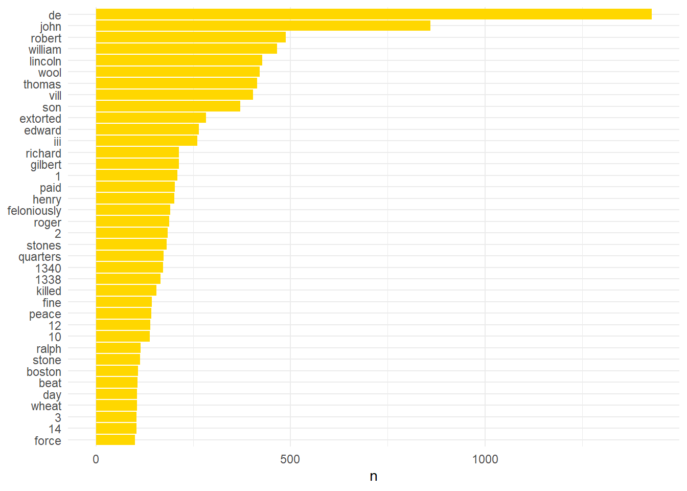
Stop! Regex Time
This plot indicates a further problem. It contains numbers and years which are very frequent. Regular expressions (regex) can be used to remove these. These are codes which can be used in place of text characteristics such as upper case letter, punctuation, or, in this case, digits.
# This removes the digits

lincs_digit_stopped <- lincs_people_stopped %>% filter(grepl('^\\D', word))
The edited data now looks more informative. The vast majority of the unique tokens in this corpus was personal names: the count of individual tokens drops to 1,641 unique words from 4,472 when they are removed. This collection of names now constitutes a useful data set which I can use to interrogate future texts. With these I could automatically identify individuals and this may be more useful than the Recogito tools when working with texts from fourteenth century England.
#This re-runs the plot filtered to only include words which occur 75 times or more.

lincs_digit_stopped %>% count(word, sort = TRUE) %>% filter(n > 75) %>% mutate(word = reorder(word,n)) %>% ggplot(aes(word, n)) + geom_col(fill="#ffd700") + xlab(NULL) + coord_flip() + theme_minimal()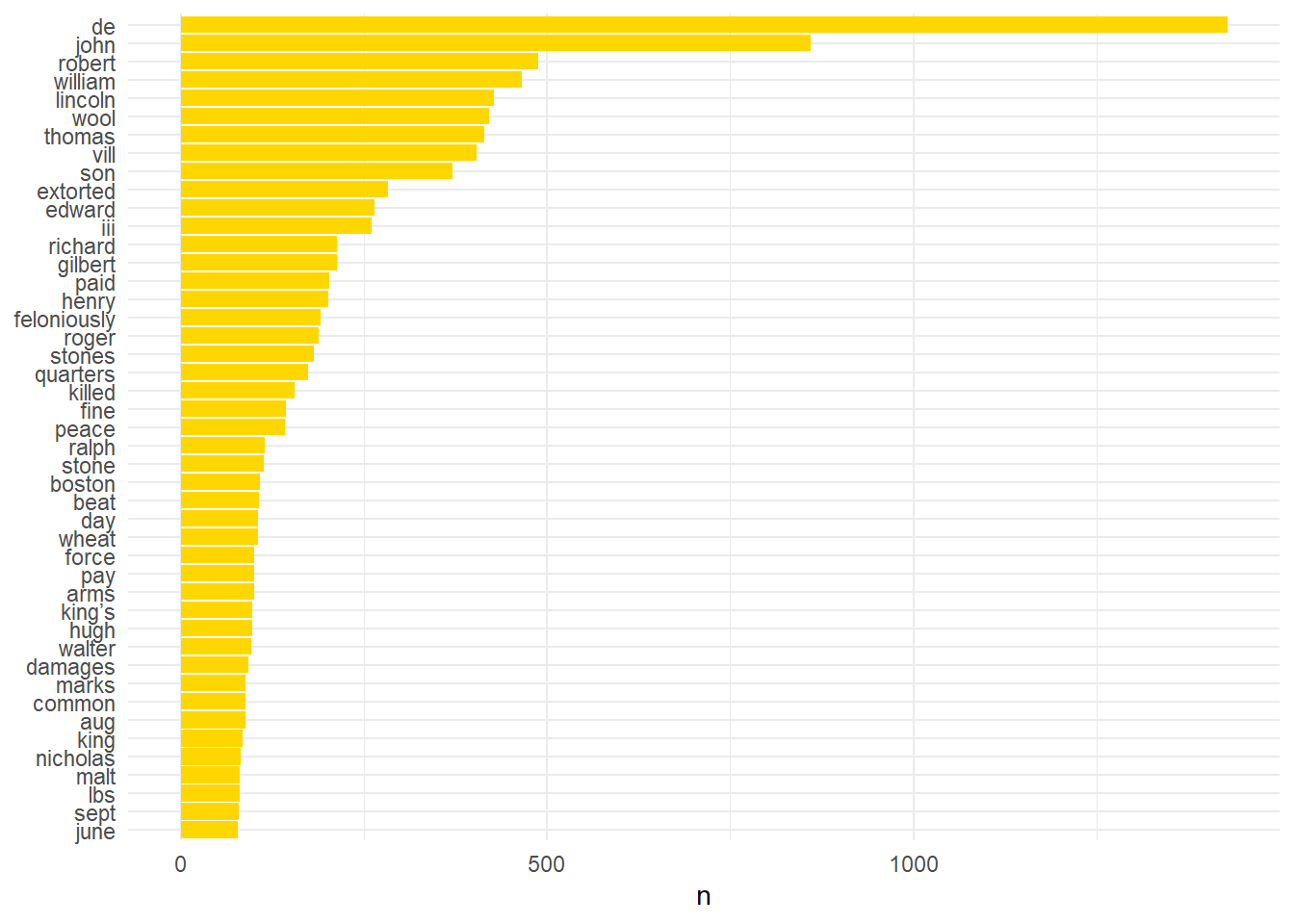
There are now several words which could be used, with context, to indicate the nature of an allegation. Wool, for example, could be utilised to tag an event as an offence involving wool. Beat, kill, or force can be used to indicate the allegation contained an accusation of violence ‘Feloniously’ however always occurs alongside another word such as theft or beat and so is less useful when it is ‘de-coupled’. This will be useful however when I interrogate this same data using bi-grams (two word pairings). It is possible, using words like ‘aug’, ‘sept’, or ‘june’ to automatically date allegations but it would require slightly more work and I don’t currently have the energy, or willpower, for that just now.
Month by Month
However, out of interest, I gathered every instance of a month name and plotted these to depict the most common months recorded in the trial. I did this by creating a data frame with all the months of the year and used inner_join() (the opposite of anti_join()) to match all the months from the data. There were six hundred cases in which allegations included some mention of a month and the resulting plot is a fairly good, although crude, indicator of when most crimes were said to have occurred.
# Create a data frame with all variations of month names
months_variations <- data.frame(
  word = c("january", "jan", "february", "feb", "march", "mar",
           "april", "apr", "may", "june", "jun", "july", "jul",
           "august", "aug", "september", "sep", "sept", "october",
           "oct", "november", "nov", "december", "dec")
)

#inner_join to find months from the data and return to a new data frame called monthsCount

monthsCount <- inner_join(lincsEventsTokens, months_variations)
Joining with `by = join_by(word)`#I also needed to format the new dataset to single variables as McLane included months in the long and short format (Jan and January). I have only included the beginning to give you an idea of how I did it. I am sure there is an easier way to accomplish this but I don't know it.
monthsCount <- monthsCount %>%
mutate(word = case_when(
word == "january" | word == "jan" ~ "jan",
word == "february" | word == "feb" ~ "feb",
word == "march" | word == "mar" ~ "mar",
word == "april" | word == "apr" ~ "apr",
word == "may" ~ "may",
word == "june" | word == "jun" ~ "jun",
word == "july" | word == "jul" ~ "jul",
word == "august" | word == "aug" ~ "aug",
word == "september" | word == "sep" | word == "sept" ~ "sep",
word == "october" | word == "oct" ~ "oct",
word == "november" | word == "nov" ~ "nov",
word == "december" | word == "dec" ~ "dec",
TRUE ~ word # This line handles any values that don't match the above conditions
))monthsReversed <- c("dec", "nov", "oct", "sep", "aug", "jul", "jun", "may", "apr", "mar", "feb", "jan")
#Plot of months
monthsCount %>% count(word) %>% ggplot(aes(x = factor(word, level = monthsReversed), y = n)) + geom_col(fill="#ffd700") + xlab(NULL) + coord_flip() + theme_minimal()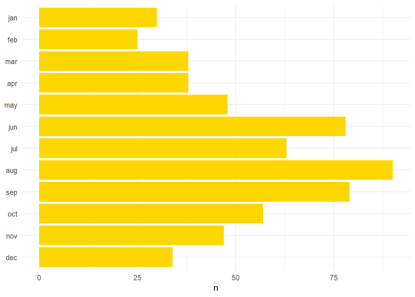
It is immediately striking that the months from June (78 occurrences) to September (79 occurrences) are the peak for alleged offences. Apparently this is a known phenomena even today: “most violent crimes against persons increase linearly with heat, while property crimes are not strongly related to temperature changes”3. It is intriguing that this is observable over six-hundred years earlier and in future I will try and see if if I can plot this time data against a categorisation of the allegations.
Let’s get toponymical
As lots of names are toponymical, especially in the fourteenth century, many place names were removed when I eliminated personal names. Fortunately Recogito also automatically labels text it thinks are place names and generates latitude and longitude. As stated earlier this requires a bit of oversight as the gazetteers it uses to carry out this analysis are not geared towards medieval English locations. In the longer term I would love to develop a gazetteer for medieval English place names but for now it requires a lot of manual oversight. Currently, to auto-generate geo-locations I use a script which queries Google map data (I have written about this elsewhere and I will migrate this over to the new site shortly). This is not perfect either but currently it is easier fix the mistakes in this process than Recogito which can be a bit convoluted. Removing the place names reduces the data set to 1,232 (c. 400) unique tokens. At this point, in order to generate a manageable amount of tokens I filtered to only include words which occur 6 or more times in the corpus and this left only 294 unique tokens.
lincs_filterOver25 <- read.csv('lincs_filterOver25.csv')

#Plot with personal names removed

lincs_filterOver25 %>% filter(n > 70) %>% mutate(word = reorder(word,n)) %>% ggplot(aes(word, n)) + geom_col(fill="#ffd700") + xlab(NULL) + coord_flip() + theme_minimal()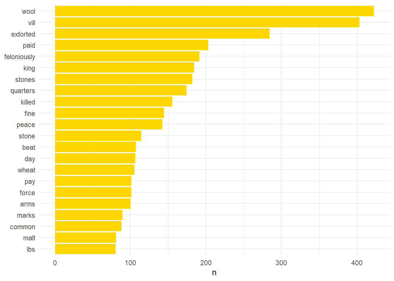
Manual Tagging
The resulting data after filtering began to resemble something which may be useful. The preponderance of wool in the corpus is due to the importance of the wool trade nationally but also particularly for Lincolnshire which produced the best wool in the country. Lincolnshire was also home to some of the most important wool merchants in the country, and perhaps continent, at this point. The majority of the references to wool relate to allegations of corrupt wool collectors who were engaged in revenue raising for Edward III in the late 1330s.
For the next step I manually added tags to each of these tokens. Words were tagged according to certain categories such as times (day, night etc), locations (house, court, fairs), as relating to allegations against officials (weighing, tax, coroner), descriptors which might indicate the nature of a crime (beat, imprisoned, stole), produce (wheat, wool, oats), livestock (pigs, horse, cattle), position (church officials, professions). Clearly there is some overlap is these categorisations. I have labelled the token ‘imprisoned’ as relating to the crimes of officials as it is usually carried out by bailiffs, sheriffs, or under sheriffs. However, in some cases this did not relate to the actions of royal officials but private individuals such as the Lincoln couple who were said to have ‘caused Walter de Toronde, lute player, living in Lincoln, to come to their house and […] imprisoned him’. However, when I use these tags to label the allegations I will be using them in conjunction with other methods which will give a more nuanced picture. Clearly this stage requires quite good familiarity with the text and its context. Utilising these tags I can generate new plots that demonstrate interesting trends.
#Plot of words associated with allegations against officials

lincs_filterOver25 %>% filter(tag1 == 'official', n > 15) %>% mutate(word = reorder(word,n)) %>% ggplot(aes(word, n)) + geom_col(fill="#ffd700") + xlab(NULL) + coord_flip() + theme_minimal()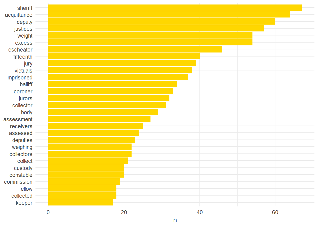
That the sheriff takes pride of place is perhaps expected due to the pivotal role of the sheriff as the keystone of royal administration in the counties. Likewise the frequency of the escheator is a result of their widespread and varied activities. Both of these officials often devolved their responsibilities onto subordinates and this is borne out in the large numbers of deputies mentioned. The prominence of words like acquittance and receivers, among others, are a result of the widespread corruption of wool collectors in the late 1330s. The prevalence of fifteenth, assessment, and assessed can be associated with tax collection. Collectors, collect, weighing, weight, excess are connected to a number of roles including wool collectors, taxers, and purveyors who supplied foodstuffs to the armies of Edward III.
The tidy text package has allowed me to pare down this corpus to a small manageable set which I will use to identify crime by particular types of officials. Hopefully this has demonstrated some of the value of text mining. In future I will outline how I used the data produced by this analysis to automatically categorise allegations. The steps I have carried out today are repeatable for any future texts of a similar nature. I have three more court rolls that have been published by local record societies and I plan to process them in a similar way. While each text will vary according to the practice and goals of the editors I can use the steps I have outlined here to remove digits, months, personal, or place names, as well as common English words. In the next post I will date all of the allegations from the corpus.
Footnotes
Silge, Julia, and David Robinson. Text Mining with R: A Tidy Approach. Boston: O’Reilly, 2017.↩︎
McLane, Bernard William, ed. The 1341 Royal Inquest in Lincolnshire. The Publications of the Lincoln Record Society, v. 78. Woodbridge, Suffolk: Lincoln Record Society; Boydell Press, 1988.↩︎
Cohn, Ellen G. ‘Weather and Crime’. The British Journal of Criminology 30, no. 1 (1990): 51–64; Also see: Butke, Paul, and Scott C. Sheridan. ‘An Analysis of the Relationship between Weather and Aggressive Crime in Cleveland, Ohio’. Weather, Climate, and Society 2, no. 2 (2010): 127–39. https://doi.org/10.1175/2010WCAS1043.1; or: Horrocks, James, and Andrea Kutinova Menclova. ‘The Effects of Weather on Crime’. New Zealand Economic Papers 45, no. 3 (December 2011): 231–54. https://doi.org/10.1080/00779954.2011.572544.↩︎